Difference between revisions of "Moore neighbourhood"
Apple Bottom (talk | contribs) (Use {{LinkMathworld}}) |
|||
| (13 intermediate revisions by 3 users not shown) | |||
| Line 1: | Line 1: | ||
{{Glossary}} | |||
[[File:Moore neighbourhood (range 1).png|framed|right|The Moore neighbourhood (in green) of a single cell]] | |||
The '''Moore neighbourhood''' is the set of all [[cell]]s that are orthogonally or diagonally-adjacent to the region of interest (the region of interest itself may or may not be considered part of the Moore neighbourhood, depending on context). For example, the Moore neighbourhood of a single cell consists of the eight cells immediately surrounding it. This neighbourhood is named after Edward F. Moore, one of the pioneers of [[cellular automata]] theory.<ref>{{Cite web|url=http://cell-auto.com/neighbourhood/moore/|title=The Moore neighbourhood|author=Tim Tyler|accessdate=June 13, 2009}}</ref> The Moore neighborhood is the neighbourhood of interest in [[Conway's Game of Life]] and all [[Life-like cellular automata]], though there are cellular automata that use other neighbourhoods such as the 4-cell [[von Neumann neighborhood]]. | |||
The Moore neighbourhood naturally extends to cellular automata in higher dimensions, for example forming a 26-cell cubic neighborhood for a cellular automaton in three dimensions. The number of cells in the Moore neighbourhood of a single cell in an n-dimensional cellular automaton is 3<sup>n</sup>-1 (Sloane's | The Moore neighbourhood naturally extends to cellular automata in higher dimensions, for example forming a 26-cell cubic neighborhood for a cellular automaton in three dimensions. The number of cells in the Moore neighbourhood of a single cell in an n-dimensional cellular automaton is 3<sup>n</sup>-1 (Sloane's {{OEIS|A024023}}). | ||
The Moore neighbourhood of a cell can be thought of as the points at a Chebyshev distance of 1 from that cell. | The Moore neighbourhood of a cell can be thought of as the points at a Chebyshev distance of 1 from that cell. | ||
==Generalizations== | |||
{{main|Isotropic non-totalistic Life-like cellular automaton}} | |||
Like in the [[hexagonal neighborhood]], [[isotropic]] cellular automata using the Moore neighbourhood can be defined using [[Hensel notation]], which was devised by [[Alan Hensel]] and represents the relative permutations of the cells using letters. | |||
{| class="wikitable" style="margin-left: auto; margin-right: auto; border: none;" | |||
| style="border: none; background: #fff;" | | |||
! 0 !! 1 !! 2 !! 3 !! 4 !! 5 !! 6 !! 7 !! 8 | |||
|- | |||
! —<small style="font-weight: normal;"> (no<br/>letter)</small> | |||
| [[File:Neighborhood 0.png]] || || || || || || || || [[File:Neighborhood 8.png]] | |||
|- | |||
! c<br/><small style="font-weight: normal;">(corner)</small> | |||
| || [[File:Neighborhood 1c.png]] || [[File:Neighborhood 2c.png]] || [[File:Neighborhood 3c.png]] || [[File:Neighborhood 4c.png]] || [[File:Neighborhood 5c.png]] || [[File:Neighborhood 6c.png]] || [[File:Neighborhood 7c.png]] || | |||
|- | |||
! e<br/><small style="font-weight: normal;">(edge)</small> | |||
| || [[File:Neighborhood 1e.png]] || [[File:Neighborhood 2e.png]] || [[File:Neighborhood 3e.png]] || [[File:Neighborhood 4e.png]] || [[File:Neighborhood 5e.png]] || [[File:Neighborhood 6e.png]] || [[File:Neighborhood 7e.png]] || | |||
|- | |||
! k<br/><small style="font-weight: normal;">(knight)</small> | |||
| || || [[File:Neighborhood 2k.png]] || [[File:Neighborhood 3k.png]] || [[File:Neighborhood 4k.png]] || [[File:Neighborhood 5k.png]] || [[File:Neighborhood 6k.png]] || || | |||
|- | |||
! a<br/><small style="font-weight: normal;">(adjacent)</small> | |||
| || || [[File:Neighborhood 2a.png]] || [[File:Neighborhood 3a.png]] || [[File:Neighborhood 4a.png]] || [[File:Neighborhood 5a.png]] || [[File:Neighborhood 6a.png]] || || | |||
|- | |||
! i | |||
| || || [[File:Neighborhood 2i.png]] || [[File:Neighborhood 3i.png]] || [[File:Neighborhood 4i.png]] || [[File:Neighborhood 5i.png]] || [[File:Neighborhood 6i.png]] || || | |||
|- | |||
! n | |||
| || || [[File:Neighborhood 2n.png]] || [[File:Neighborhood 3n.png]] || [[File:Neighborhood 4n.png]] || [[File:Neighborhood 5n.png]] || [[File:Neighborhood 6n.png]] || || | |||
|- | |||
! y | |||
| || || || [[File:Neighborhood 3y.png]] || [[File:Neighborhood 4y.png]] || [[File:Neighborhood 5y.png]] || || || | |||
|- | |||
! q | |||
| || || || [[File:Neighborhood 3q.png]] || [[File:Neighborhood 4q.png]] || [[File:Neighborhood 5q.png]] || || || | |||
|- | |||
! j | |||
| || || || [[File:Neighborhood 3j.png]] || [[File:Neighborhood 4j.png]] || [[File:Neighborhood 5j.png]] || || || | |||
|- | |||
! r | |||
| || || || [[File:Neighborhood 3r.png]] || [[File:Neighborhood 4r.png]] || [[File:Neighborhood 5r.png]] || || || | |||
|- | |||
! t | |||
| || || || || [[File:Neighborhood 4t.png]] || || || || | |||
|- | |||
! w | |||
| || || || || [[File:Neighborhood 4w.png]] || || || || | |||
|- | |||
! z | |||
| || || || || [[File:Neighborhood 4z.png]] || || || || | |||
|} | |||
For instance, B2-a/S12 (the [[Just Friends]] rule) indicates that a dead cell will be born with 2 neighbors, except when they are adjacent, and that a live cell will survive with 1 or 2 neighbors in any configuration. | |||
==Higher ranges== | ==Higher ranges== | ||
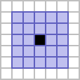
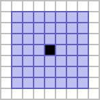
The Moore neighbourhood can also be defined with a higher ''range''; that is, so that it captures cells that are further than one cell away from the region of interest. The standard Moore neighbourhood has range 1. The Moore neighbourhood of range 2 is the set of all cells that are orthogonally or diagonally-adjacent to the Moore neighbourhood itself. The Moore neighbourhood of range n can be defined recursively as the set of all cells that are orthogonally or diagonally-adjacent to the Moore neighbourhood of range n-1. The number of cells in the Moore neighbourhood of range n is given by (2n+1)<sup>2</sup>-1 (Sloane's [ | The Moore neighbourhood can also be defined with a higher ''range''; that is, so that it captures cells that are further than one cell away from the region of interest. The standard Moore neighbourhood has range 1. The Moore neighbourhood of range 2 is the set of all cells that are orthogonally or diagonally-adjacent to the Moore neighbourhood itself. The Moore neighbourhood of range n can be defined recursively as the set of all cells that are orthogonally or diagonally-adjacent to the Moore neighbourhood of range n-1. The number of cells in the Moore neighbourhood of range n is given by (2n+1)<sup>2</sup>-1 (Sloane's {{OEIS|A033996}}). | ||
==Symmetries== | |||
{{main|Symmetry}} | |||
The Moore and von Neumann neighbourhoods rely on a different grid than the [[hexagonal neighbourhood]] and thus features a different set of inherent symmetries when dealing with [[isotropic]] rules: | |||
* C2_1 | |||
* C2_2 | |||
* C2_4 | |||
* C4_1 | |||
* C4_4 | |||
* D2_+1 | |||
* D2_+2 | |||
* D2_x | |||
* D4_+1 | |||
* D4_+2 | |||
* D4_+4 | |||
* D4_x1 | |||
* D4_x4 | |||
* D8_1 | |||
* D8_2 (only occasionally preserved) | |||
* D8_4 | |||
==Image gallery== | ==Image gallery== | ||
| Line 12: | Line 87: | ||
|- | |- | ||
|[[Image:Mooreneighbourhood_eater1.png|framed|left|The Moore neighbourhood (in green) of an [[eater 1]]]] | |[[Image:Mooreneighbourhood_eater1.png|framed|left|The Moore neighbourhood (in green) of an [[eater 1]]]] | ||
|[[ | |[[File:Moore neighbourhood (range 2).png|framed|left|The Moore neighbourhood of range 2 of a single cell]] | ||
|[[File:Moore neighbourhood (range 3).png|framed|left|The Moore neighbourhood of range 3 of a single cell]] | |||
|} | |} | ||
==See also== | ==See also== | ||
*[[Zone of influence]] | * [[Neighbourhood]] | ||
** [[Hexagonal neighbourhood]] | |||
** [[Margolus neighbourhood]] | |||
** [[von Neumann neighbourhood]] | |||
** [[Triangular Moore neighbourhood]] | |||
** [[Triangular von Neumann neighbourhood]] | |||
** [[Euclidean neighbourhood]] | |||
** [[Circular neighbourhood]] | |||
* [[Zone of influence]] | |||
==References== | ==References== | ||
| Line 22: | Line 106: | ||
==External links== | ==External links== | ||
{{LinkWikipedia|Moore_neighborhood}} | {{LinkWikipedia|Moore_neighborhood|name=Moore neighborhood}} | ||
{{LinkLexicon|lex_m.htm#mooreneighbourhood}} | |||
{{LinkMathworld|MooreNeighborhood.html|pagename=Moore neighborhood}} | {{LinkMathworld|MooreNeighborhood.html|pagename=Moore neighborhood}} | ||
__NOTOC__ | |||
Revision as of 01:13, 25 August 2019
The Moore neighbourhood is the set of all cells that are orthogonally or diagonally-adjacent to the region of interest (the region of interest itself may or may not be considered part of the Moore neighbourhood, depending on context). For example, the Moore neighbourhood of a single cell consists of the eight cells immediately surrounding it. This neighbourhood is named after Edward F. Moore, one of the pioneers of cellular automata theory.[1] The Moore neighborhood is the neighbourhood of interest in Conway's Game of Life and all Life-like cellular automata, though there are cellular automata that use other neighbourhoods such as the 4-cell von Neumann neighborhood.
The Moore neighbourhood naturally extends to cellular automata in higher dimensions, for example forming a 26-cell cubic neighborhood for a cellular automaton in three dimensions. The number of cells in the Moore neighbourhood of a single cell in an n-dimensional cellular automaton is 3n-1 (Sloane's ![]() A024023).
A024023).
The Moore neighbourhood of a cell can be thought of as the points at a Chebyshev distance of 1 from that cell.
Generalizations
- Main article: Isotropic non-totalistic Life-like cellular automaton
Like in the hexagonal neighborhood, isotropic cellular automata using the Moore neighbourhood can be defined using Hensel notation, which was devised by Alan Hensel and represents the relative permutations of the cells using letters.
For instance, B2-a/S12 (the Just Friends rule) indicates that a dead cell will be born with 2 neighbors, except when they are adjacent, and that a live cell will survive with 1 or 2 neighbors in any configuration.
Higher ranges
The Moore neighbourhood can also be defined with a higher range; that is, so that it captures cells that are further than one cell away from the region of interest. The standard Moore neighbourhood has range 1. The Moore neighbourhood of range 2 is the set of all cells that are orthogonally or diagonally-adjacent to the Moore neighbourhood itself. The Moore neighbourhood of range n can be defined recursively as the set of all cells that are orthogonally or diagonally-adjacent to the Moore neighbourhood of range n-1. The number of cells in the Moore neighbourhood of range n is given by (2n+1)2-1 (Sloane's ![]() A033996).
A033996).
Symmetries
- Main article: Symmetry
The Moore and von Neumann neighbourhoods rely on a different grid than the hexagonal neighbourhood and thus features a different set of inherent symmetries when dealing with isotropic rules:
- C2_1
- C2_2
- C2_4
- C4_1
- C4_4
- D2_+1
- D2_+2
- D2_x
- D4_+1
- D4_+2
- D4_+4
- D4_x1
- D4_x4
- D8_1
- D8_2 (only occasionally preserved)
- D8_4
Image gallery
 The Moore neighbourhood (in green) of an eater 1 |
See also
References
- ↑ Tim Tyler. "The Moore neighbourhood". Retrieved on June 13, 2009.
External links
- Moore neighborhood at Wikipedia
- Moore neighbourhood at the Life Lexicon
Moore neighborhood at Wolfram Mathworld


